Exploring the Data
The dataset includes information for 100,000 policies. For the policy data, we have each policy's monthly premium, enroll date, and cancel date (if applicable). We also have claim data for these policies, including claim date, dollar amount for a claim, and the amount payed for the claim. This seemingly small amount of data provides an extreme amount of information.
Starting with the policy data, we quickly see there are ~13,000 cancellations,
leaving us with a little over 1000 cancellations/month. This will be an
important check in our final analysis. The enroll
dates span from December 2000-December 2016, with cancel dates spanning through
2016, which tells us how this data was selected.
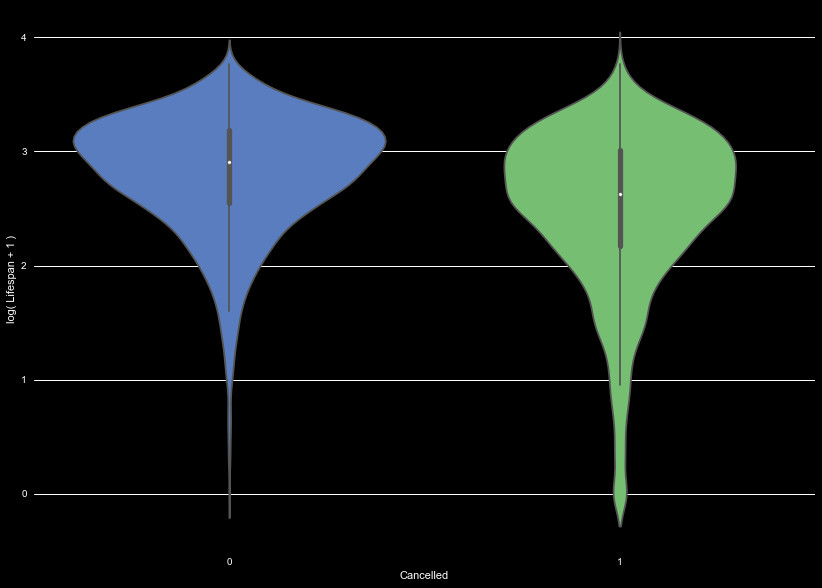
We define the lifespan of a policy
holder as the time between enrollment and cancellation of the policy, or,
the time between the enroll date and the end of our data set. We see the
kernel distribution of the lifetime of policies in Figure 1. The policies
without cancellations show a fairly even distribution between 30 and 400 days,
this demonstrates most of the accounts we have to predict on are less than about
a year and half old. Of the accounts that cancel, most cancel relatively early,
rather than when the account has existed for a long time.
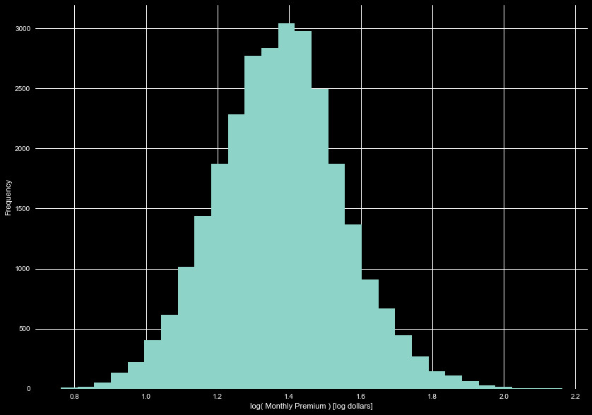
There are 5 policies with no monthly premium. These are policies we need to predict,
and we don't have claim information for them. We will have to fill these with the
median premium for the time being. Figure 2 shows the log distribution of the monthly
premiums. This shows a fair lognormal trend, centered around $30 dollars a month.
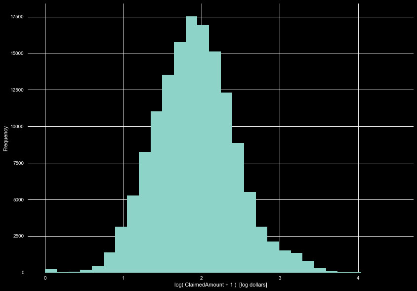
A cursory exploration of the claims set show ~145,000 claims, averaging about
1.5 claims per policy. Interestingly, we see a negative claim amount. The amount
paid out was 0, and there are numerous claim with 0 value. We will set this negative
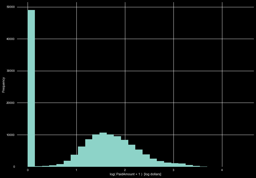
value as 0, for now. Fortunately, we see no payments that are greater than the
claimed amount. Figure 3 shows the distribution of claimed amounts, and Figure 4 the
distribution of paid amount.
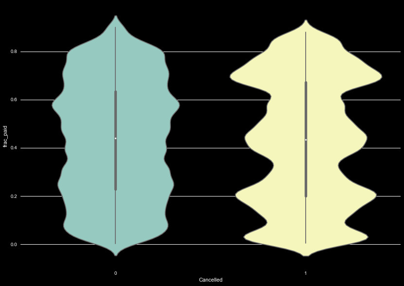
Here we can begin creating features. One interesting feature may be the
fraction of claims paid. We do this by totaling the amount of claims per
policy, and the total of the amount paid, and dividing the total paid by
the total claims per policy. It's useful to break this up by Canceled and
uncancelled policies and compare. We show this as another kernel density
plot in Figure 5. For uncancelled policies, there is a relatively even
spread. Interestingly, the Canceled policies show peaks at a few values,
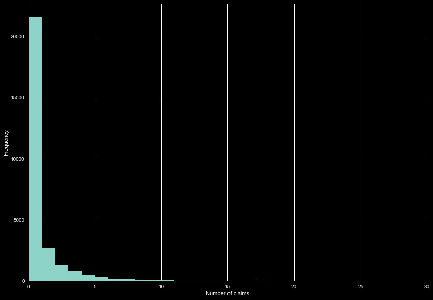
Next, we can look at the number of claims made per policy. Upon exploration,
we see there can be multiple claims per day. While we could leave this as is,
there is some benefit to reducing this value so there is only one claim in a
day. This changes multiple claims, to claim "events". Easily one event could
lead to multiple claims (multiple shots, sedatives + operation, etc.), whereas
they can be simplified to related to the same cause (needs their immunizations,
injured a leg, etc.). To distinguish between someone who uses the insurance a
lot and someone who just had to individually claim a lot of items for one event,
we will only permit one event per day. Claims may still be related on low day
timescales, but this is unavoidable. With this as our definitions for the
number of claims, we see the distribution of claims in Figure 6. When combining
claims per day, we lump the claimed amount and payed amount together, in
future analysis.
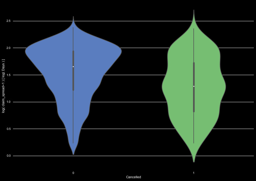
With our claims set as events, we can look at the spread of time between
events for people with multiple claims. For every policy with multiple claims,
we find the difference between these claims for each policy in days, and fit
a normal distribution to the spread in days.
While we do not assert this distribution should follow a Gaussian distribution
for an individual policy, the standard deviation gives an idea as to how
often a policyholder will use their insurance. We call this standard deviation
the claim spread, and it varies wildly. We show another kernel density plot
for the claim spread, between Canceled and non-Canceled policies in Figure 7.
We see the Canceled policies show a fairly even distribution in the claim
spread, whereas policies that don't cancel show a long term peak. This has a few
possible interpretations. As many of the canceled policies don't have a long lifetime,
they are less likely to have a long distribution in days between claims. Also,
if a customer is less likely to file claims on long timescales, they may choose to
cancel.
We use these features in our machine learning algorithm. When fed into the
algorithms, we use z scaling to scale normal features, and min/max normalization
on non-normal features. We won't go into further detail, and instead will focus
on more interesting analysis. The next step:
Survival Analysis.