Training the Machine Learning Algorithms
With our features generated and scaled, we are now free to begin training different machine learning algorithms, and select which to use for our final predictor. It is here that we implement a fundamental, bad assumption: the trend in the closing stock price is only dependent on the features we have selected, and no other external factors. We make this assumption for simplicity, we are trying to predict trends, not be able to nail down the exact stock price after the third quarter earnings are announced, just before the yearly trade show for a company. It is more of a tool that could be used with that external model to make investing decisions.
There are two important things that fall out of making this assumption, in regards to training the algorithm. First, we are able to train on all of our quote data over the full time window. Ordinarily with time series data, it is vital to train on the earliest data, and train on the latest data. With our assumption, this goes away, since past data is in the features we include, and we assume that information is all we need to determine future trends. Second, as we can train on the most recent data, we include the most recent data in the market, and don't have to worry that our data is trained on markets from 2-10 years in the past, which may behave very differently.
Model Selection and Tuning
The data was shuffled and split into an 80/20 training/test samples. The target variables were the percentage increase/decrease in the rolling mean of the stock price for different day means. We used Python's scikit-learn package to generate our machine learning algorithms, and tuned the hyperparameters of the estimators using cross validation on different folds of the training data.
We decided to test several machine learning regressors for this project, including SVM, Random Forest, Multi Layered Perceptron, a Bagging Regressor, and finally an Adaboost Regressor. These were each selected for their potential strengths with this kind of data. Support vectors tend to perform well with large amounts of continuous data. A Random Forest may simulate the way an investor may thing, comparing multiple traditional estimators to determine a future trend. Similarly, neural nets have proved excellent at combining a large amount of chaotic data to make accurate predictions, adding the Multi Layered Perceptron to our list. Bagging Regressors are another good choice when dealing with noisy data, combing multiple other regressors. Finally, Adaboost is an excellent choice for noisy data, adapting weights and repeatedly refitting to provide better results.
We also considered implementing a model that included principle component analysis. As many of our features only differed in the number of days the variable was calculated over, there is huge overlap in the information contained. We thus fit models with and without PCA implementation, reducing the dimensionality of the momentum variables from 5 to 2, the Bollinger Band variables from 5 to 2, and the RSI variables from 2 to 1 (using a 90% threshold for information).
We further tested whether it would be worth attempting to predict the rolling mean change, not the percent change.
For the initial model selection, we compared the predictions for the
5 day and 15 day rolling means. This subset was chosen to be a simple
test of short and long term predictions. The mean square error of the
predictions, with PCA and non-percentage variations, can be seen in
table 1.
| N days Rolling Mean | SVR | SVR, PCA | SVR, Abs | RFR | RFR, PCA | RFR, Abs | MLP | MLP, PCA | MLP, Abs | Bag | Bag, PCA | Bag, Abs | Ada | Ada, PCA | Ada, Abs |
|---|---|---|---|---|---|---|---|---|---|---|---|---|---|---|---|
| 5 Day | 0.00145 | 0.00133 | 33.5 | 0.00128 | 0.00133 | 27.4 | 0.00135 | 0.00141 | 24.3 | 0.00129 | 0.00133 | 25.5 | 0.00125 | 0.00130 | 27.9 |
| 15 Day | 0.00294 | 0.00270 | 81.8 | 0.00273 | 0.00265 | 63.9 | 0.00293 | 0.00304 | 64.2 | 0.00275 | 0.00270 | 62.9 | 0.00263 | 0.00255 | 64.3 |
Looking at the table, there is no clear benefit from including PCA to
our pipeline. Without an added benefit, we chose to omit PCA, to include
as much information as possible, and decrease data reduction time.
Less obvious, is whether or not the absolute change in rolling mean provides
different results than a percent change in rolling mean. A percent change
is easy to interpret as MSE, however prices can vary wildly, making a MSE
of say, $25.5, harder to interpret. A few percent MSE seems smaller than
a thirty dollar MSE, but let's examine the results in more detail.
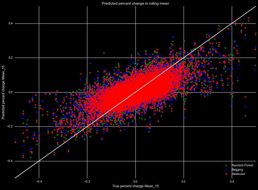
Generally, Adaboost demonstrated the best performance, followed by the Bagging
regressor, then the Random Forest. Figure 1 shows the predicted 15 day percentage
increase, as a function of the true 15 day percentage increase, for our test
dataset. They all demonstrate the same general trends, over predicting the
downward trends, and under predicting the upward trends, but overall much of the
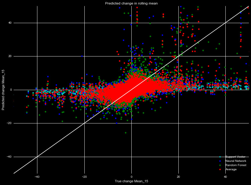
variability is captured. Figure 2 shows the same data, but for the models predicting
absolute changes in the predicted price. Clearly, these algorithms fail, so
we will utilize the percent change model. Specifically, we will adopt the
Adaboost regressor, which scored the best for both the 5 and 15 day tests.
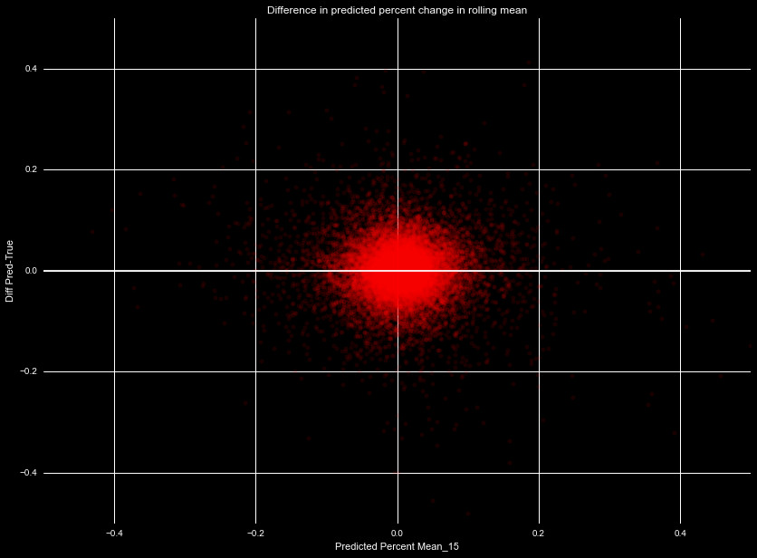
One may be inclined to fit a linear regression on the results in Figure 1,
and transform the results so they fit on a 1:1 line. This is would however
result in worse performance of our algorithm. To understand why, we plot in
Figure 3 the difference in the predicted percent change and true percent
change, as a function of the predicted change for the 15 day mean. There is
clear symmetry in the uncertainty, a symmetry that is necessary to have unbiased
results, as we are assuming the predicted value as the true value. If we
attempted further transform, it would skew this error, and lead to biased results.