Results
With the interpolation scheme set up, we are now able to predict the closing price for days between our rolling mean predictions, and compare the results with the actual closing price.
We start by predicting the rolling means of four new stock quotes
we did not train on, GE, KMB, MMM, and MU. These represent diversity
in both industry and prices. We show a mixture of results in
Figures 1-5, for different stocks, timeframes, and rolling means.
Note the individual scales in the left panel vary by plot, but
all of the fractional differences share the same scale.
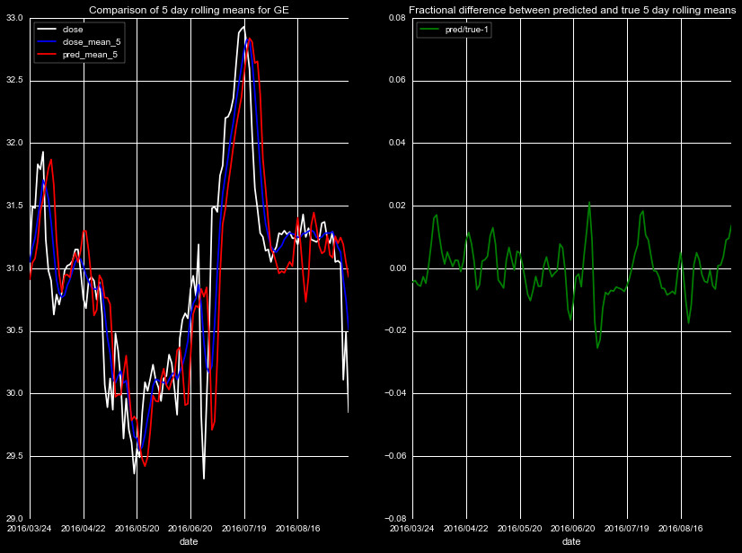
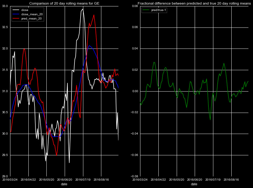
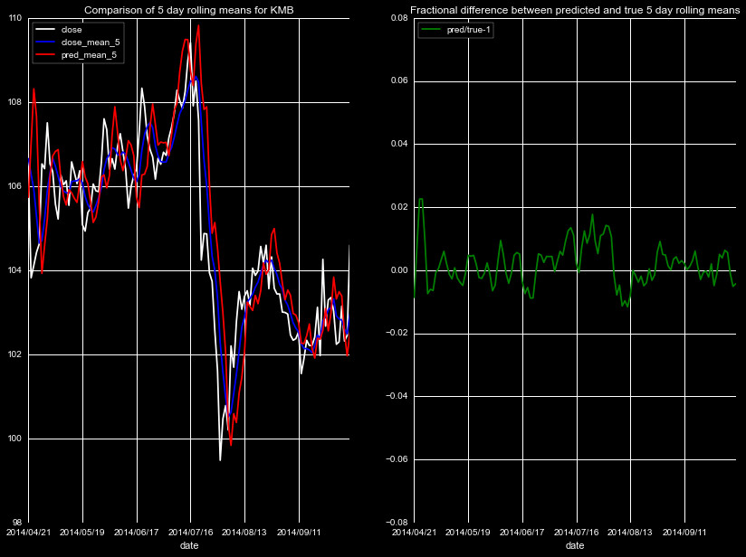
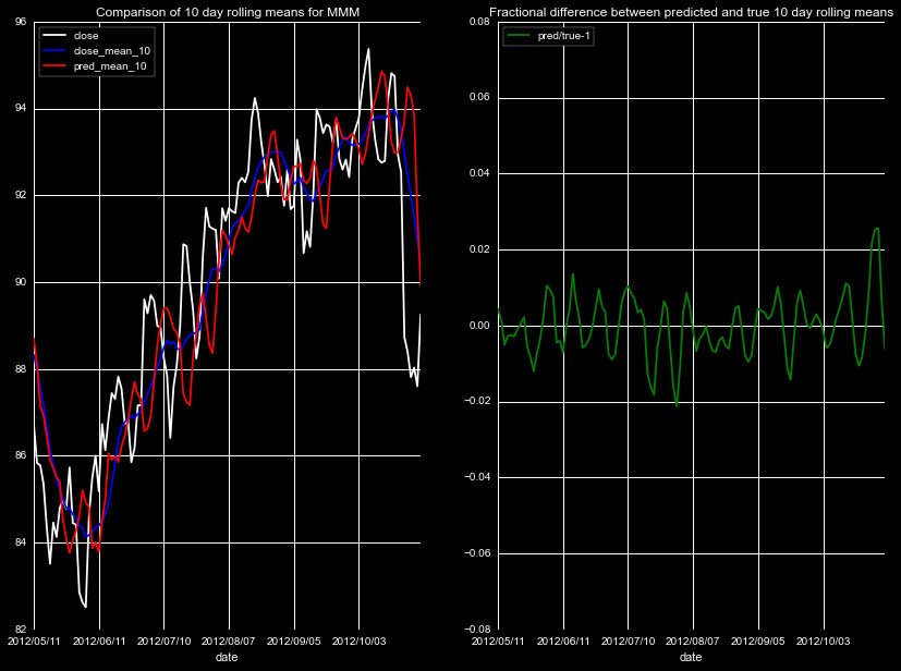
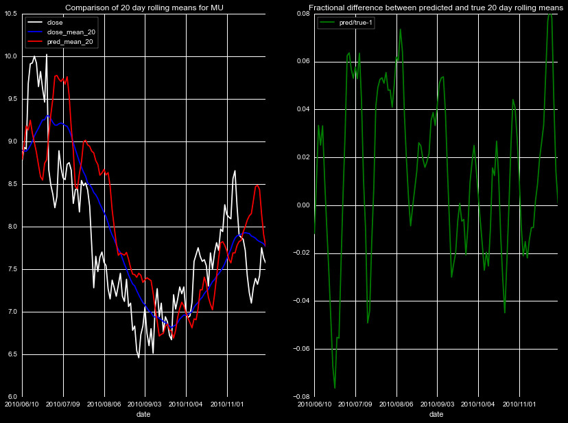
The results are mixed, there is clear noise in the predictions, and the
magnitude of the effect is dependent on the magnitude of the closing price.
We use the fractional difference for most of our error analysis, as the
price variation across 10 years will induce a bias. For example, if 10 years
ago the price was $20 with variations on the scale of $1, that is larger swing
than a $200 stock with a change of $1. An absolute variation of $1
is significantly less of a return in the later case, hence the preference for
the fractional change. Both are nonetheless good metrics.
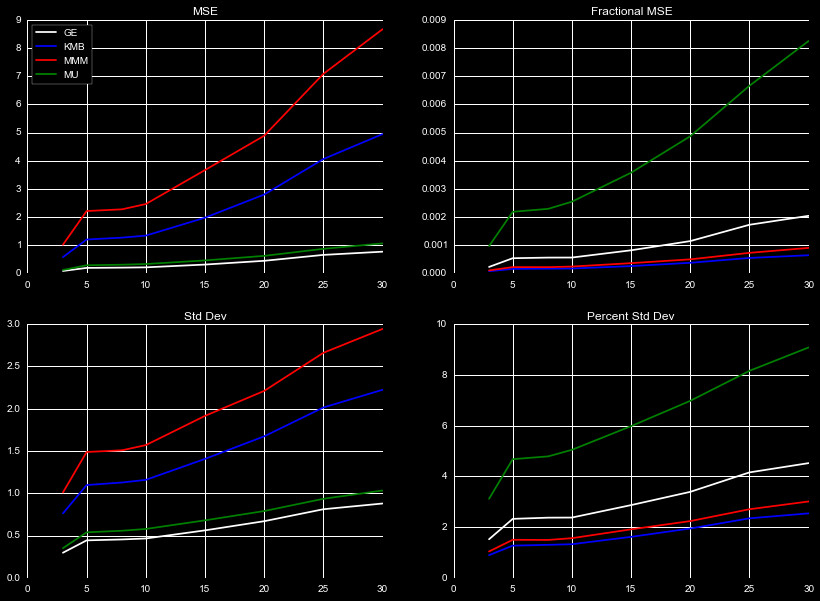
We show different metrics for the difference between the predicted rolling means and true rolling means in Figure 6. The easiest to interpret is the standard deviation, where 1 standard deviation contains roughly 68% of the data. That means for MU at 30 days, 68% of the predictions fall roughly within a dollar of the true rolling mean. MMM by this point appears worse, with a 3 dollar difference. If we look at the standard deviation using percentage differences, for MU we see that this actually constitutes almost a 9% difference in price, which is a poor predictor, whereas for MMM this is only a 3% difference.
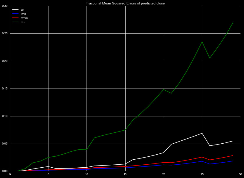
We use the rolling mean predictions and our interpolation scheme to predict
daily values for our subset of test quotes.
The fractional mean squared error is shown in Figure 7, averaged for each day
over all predictions. We see for KBM and MMM, the fraction mean squared error
is quite good. Even thirty days out, the FMSE<0.03, considering the simplicity
of our algorithm and poor assumptions, this is an excellent result. Even for
GE, with a FMSE that increases more quickly after 15 days, we see a fair
value for FMSE. The behavior of the FMSE for MU is significantly worse, with the
error skyrocketing above the others to extremely high values.
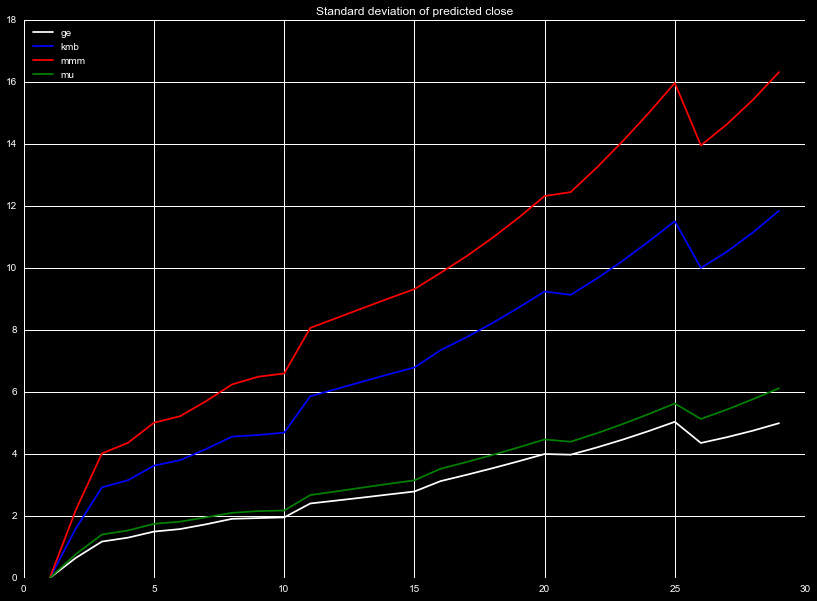
We show the absolute standard deviation of the price in Figure 8. The standard deviation is the square root of the MSE. Here we see results that are at first glance, contradictory to what we saw in Figure 6. The high fractional variation of mu but low standard deviation relative to other quotes is due to this stock having a lower closing price than the others. KMB and MMM however have higher relative prices, leading to lower fractional MSE, even with their higher standard deviations. It is vital to consider both metrics when measuring the effectiveness of the ML algorithms.
Conclusion
In conclusion, we generates a machine learning algorithm, that predicts future changes in rolling means using traditional stock predictors and indicators. We unfold the predicted rolling means to interpolate values between our predictions. Predictions of the values tested on independent stock quotes demonstrate fairly good predictive power for some stocks, for short term predictions, but overall there is large variation that makes our algorithm unreliable for long term forecasting.
While unreliable for forecasting, given the simplicity of the model and poor assumptions we intentionally made, and the the difficulty of predicting closing stocks prices and their high volatility, I am very happy with the model performance. There is lots of room for the improvements, and this is a model I intend on updating with time.