Building a model with TensorFlow
Now, we will build a deep learning model with TensorFlow. Whereas Sklearn has optimizers, cost functions, and all tuning parameters combined in a single Multi Layered Perceptron function, TensorFlow requires the user to combine these functions on their own. This makes the process more tedious, however allows more flexibility in the model, and allows including things unavailibly in Sklearn, such as dropout layers.
We construct Tensorflow models to match the Sklearn models, using rows/columns or the image itself as input. We further use these models to outline the parameter values for our model, as parameter tuning in Tensorflow is significantly more difficult than in Sklearn, but manually test tuning of parameters to optimize predictions.
Image Model
First, we attempt to implement a model matching the image analysis, a 3x3 blurred image PCA (for details, see the Sklearn Model page. The model uses an Adam solver with tanh activation, a learning rate of 5*10-3, regularization alpha of 10-3, momentum of 0.75, and hidden layer sizes of 500, 300, 350, 500, and 450. This model performs poorly, with only 82.4% accuracy.
We manually alter parameters, and find these parameters appear optimal for this model. We test varying the activation function between relu and tanh, and the solver of Adam and SGD. We also try introducing dropout layers. We find the most successful model to be an Adam solver with tanh activation, as it was in the Sklearn model. One thing we can implement in TensorFlow that is absent in Sklearn is dropout layers, so we attempt to improve the model by adding dropout layers. Manually adding layers, we find our best option is a single dropout layer after the first hidden layer dropping 15% of the nodes.
The Sklearn model rolls in with a total accuracy of 95%. By comparison, the TensorFlow model finishes with an accuracy of 91%. Considering the extra effort that goes in to constructing a model in TensorFlow, this bodes poorly for the rest of the analysis.
Row and Column Sum Model
Next, we generate a model based on the normalized row/column sum. We use an Adam solver with tanh activation function, with an initial learning rate of 9*10-4, and regularization of 10-3. We use 5 hidden layer of size 275, 350, 400, 500, and 450. We start without any dropout layers, as it is in the Sklearn model.
Again, we find altering the initial parameters shows no improvement in the model. Introducing a dropout layer after the first 500 layers, where 15% of the points are dropped, cause nearly a 2% increase in the accuracy score, so we adopt this into the model.
Comparing the Sklearn and TensorFlow models, we see Sklearn has an accuracy of 90%, and TensorFlow maxes out at about 80%. This is significantly worse performance, hopefully by combining the models the TensorFlow model will be able to match the Sklearn.
Combined Model
Both of these models show worse performance than their Sklearn counterparts. This may be due to slight difference in how the neurons are constructed, or the Sklearn function uses better optimization that converges more quickly. It could also be a combination of these, and the fact I am manually optimizing, the combination of which causes the model to not be optimized. This is the most likely scenario.
The final chance for TensorFlow to demonstrate itself as the superior model is by combining the data sets. We implement the Sklearn model, which uses and Adam solver and tanh activation. The learning rate is 7*10-4, momentum is 0.82, regularization constant of 2*10-4, and hidden layer sizes of 175, 300, 225, 275, 315, and 180. This model starts with an accuracy of 74%, significantly below the Sklearn model of 97%.
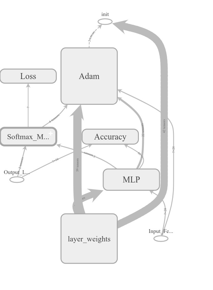
Figure 1: The final TensorFlow model graph visualization. This is a useful tool for
visualizing the flow of data using tensors. Accuracy and softmax/loss are used to
score our model, but the flow from the Multi Layered Perceptron to the Adam solver
and weights are clearly illustrated here.
This model performs slightly better when using relu, approximately 2% higher accuracy, so we adopt this activation function, deviating from the Sklearn framework. Furthermore, a faster learning rate was highly beneficial in model convergence, a rate of 10-2 leads to faster convergence and 7% increase in accuracy. As in the other TensorFlow models, a dropout layer after the first hidden layer causes a significant improvement upon the accuracy, dropping roughly 15% of the neurons. This boosted the model to a total accuracy of 93% on the test data.
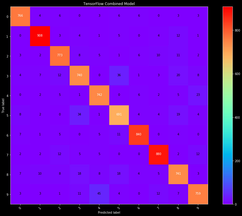
Figure 2: The final TensorFlow model confusion matrix. While this model
performs fairly well, there are clear misclassifications, and the 93%
accuracy does not compete with the 97% of the Sklearn model.
Though much of the issue with the TensorFlow model is likely due to personal inexperience in optimization, the effort required to make this model match the other models is not worth the possibility of even a 1% improvement at that high of accuracy. There are improvements that can be made to the Sklearn model that would require significantly less effort than reworking the entire TensorFlow model for better optimization. Therefore, moving forward, I will focus on the much simpler Scikit-Learn models in constructing a final model for predictions.
We finalize our model and predictions in building a final model.