Data Exploration
We will start with some basic exploration of the data set. This is a pretty straightforward project, and we do not want to spend too much time going into the simple preprocessing details, so this section will be brief.
There are 42,000 images in the data set. Each pixel is given as a value between 0 and 255, which is standard for color values. We choose to split these into a test and training data set. We will use the same split across all of our exercises.
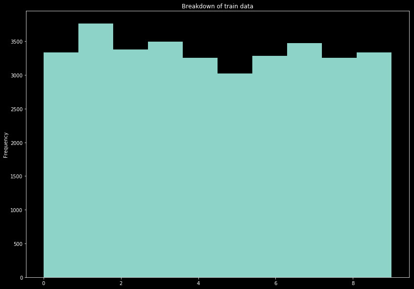
We show below the distribution in the split between test and train data.
The histogram x axis is simply the label for drawn numbers.
 |
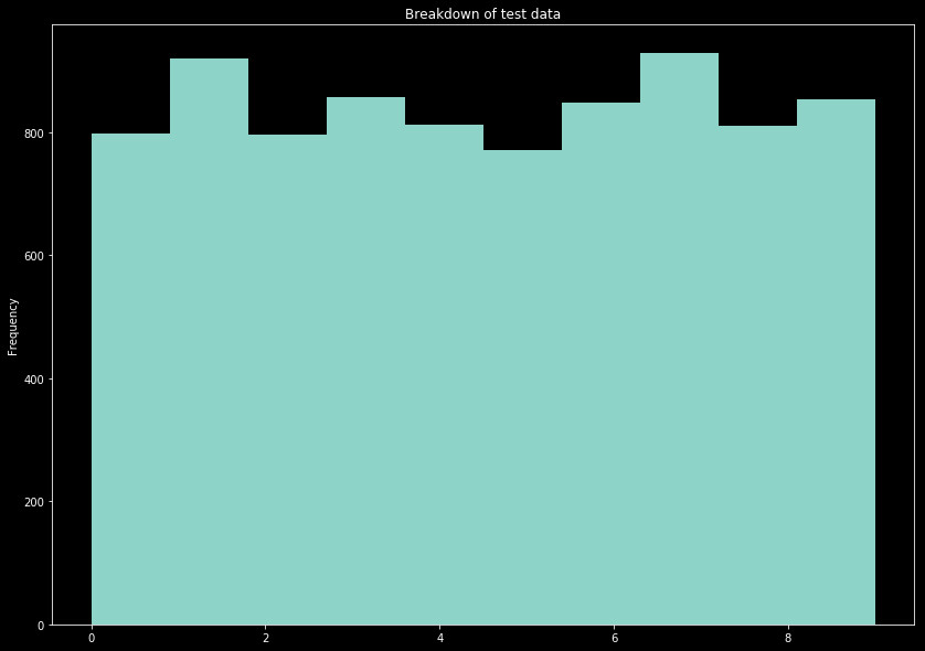 |
Ideally the data would posses an even amount of all labels. This is not the case, however. Since there is not a perfect split between the numbers in the data set, all we are looking for is a relatively even spread of the numbers between both the train and test sets. Sure enough, this split provides a pretty even distribution across both sets, with relatively consistent patterns.
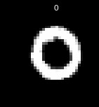
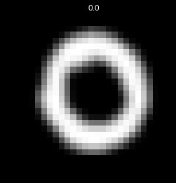
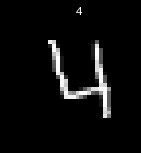
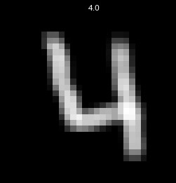
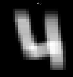
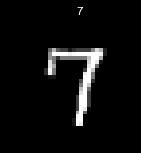
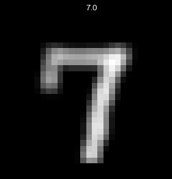
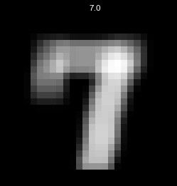
Now let's check the raw data. We show a sample of the 28x28 pixel inverted color images below. We include convolutions of these images with a 3x3 and 5x5 blur kernels. Blurring is an important step to include, as data will be less dependent on pixel to pixel variations, and it will reduce the overall dimensionality of the data.
| Raw Image | 3 x 3 Blur | 5 x 5 Blur |
|---|---|---|
 |
 |
 |
 |
 |
 |
 |
 |
 |
The last thing we will do for exploration, will be to track the explained variance using principle component analysis. Despite some dimensionality reduction from blurring, we still have hundreds upon hundreds of variables to consider. The blurring serves more to reduce some of the small scale variation, where PCA can capture some of the collective features. Below we show the explained variance, and cumulative explained variance of the smoothed 3x3 image per number of axes. We show the axis number on the x axis, and only show the first 100 axes.
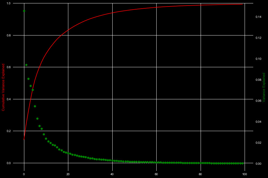
We can see that about 40 features capture about 95% of the explained variance. For our model, we will only choose to use about 25 features, which captures 85%. This reduces nearly 800 original dimensions to only 25.
We begin model building in the next section, building a model with sklearn.