Building a model with Scikit-Learn
Now we will construct the framework of our model, using Scikit-Learn. This python package contains numerous machine learning models, and we will use the Multi Layered Perceptron Classifier to construct our Neural Network. Since this is a pre-canned routine, it will make shaping a model easier than having to do things by hand, as is the case with Tensorflow.
For each of the models we construct, we train with cross validation on the same 80% of the data, and test on the same 20% of the data. As we will see, the models all have high performance, so we chose this split to leave a large chunk of data to test on. Indeed, some of the models demonstrated an accuracy of 90% when trained on less than 20% of the data, which highlights the strengths of neural networks.
Blurred Pixel PCA Model
We start by fitting a model to the PCA of the image itself, as seen in exploration. We use 25 of the hundreds of features, capturing 85% of the information. Furthermore, we use the sklearn GridsearchCV for the cross validation. Since we will be combining models later, we do not need to spend much time training the model for high accuracy now.
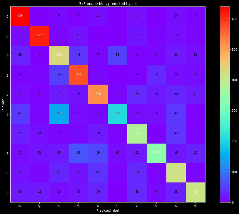
Below, we show the results for our best NN classifier, in the form of a confusion matrix. A confusion matrix is an ideal tool for visualizing multi label classifications. The confusion matrix shows the true label on the y axis, and the prediction on the x axis, with each bin as the count for our test data set. If we created a perfect classifier, every prediction would match the true label, and the only values would lie across the diagonal.
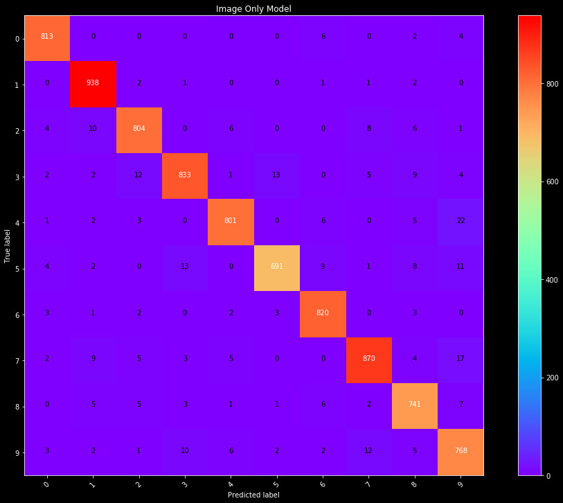
Figure 1: Confusion matrix for predictions on the test data set, from a
Neural Network. The model was fit on a PCA of the blurred images.
We see our very simple model performs very well. Most values lie on the diagonal, with low off diagonal values. We see some fives are classified as threes, sevens as nines, and nines as fours. With a little knowledge of the shapes of these numbers, these are quite reasonable mistakes for our classifier to make, considering variations in handwriting. The overall accuracy of this model (correct labels / total) is 95%.
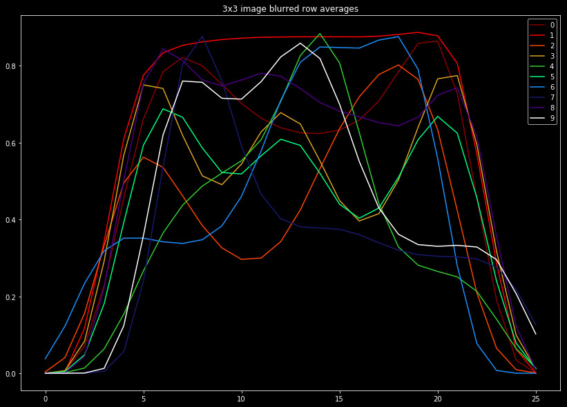
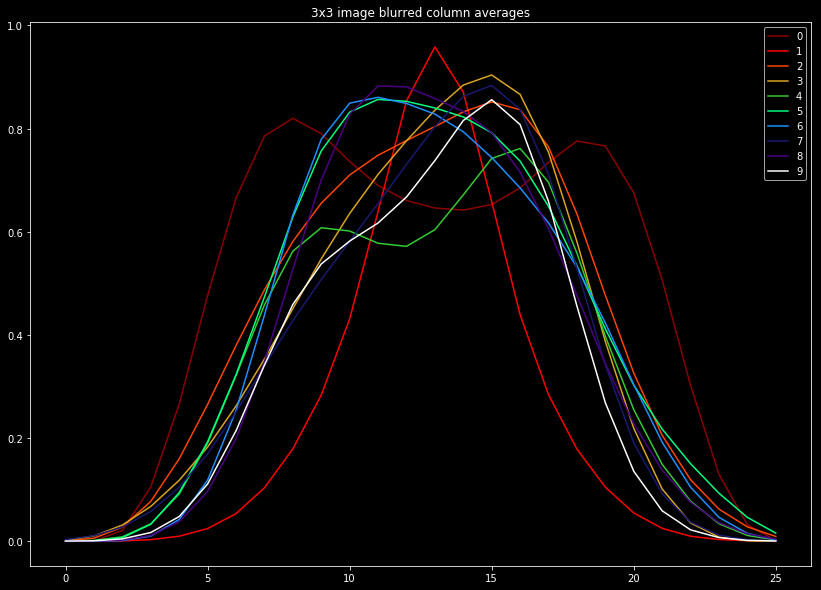
Row and Column Sum Model
Next we consider modeling the data in a completely separate way. After blurring, we sum the pixels by rows and columns, and normalize these values from 0 to 1. This gives a measure as to how the features are spread out in each dimension. For something like a zero, we would expect relatively constant values in both directions, due to symmetry. A one however, would have relatively constant value across rows, but a spike in the columns towards the image center.
To illustrate this, we plot these values averaged across our data set in the following two figures. The plots are busy, however we find it valuable to include the shape of every label, for comparison.
 |
 |
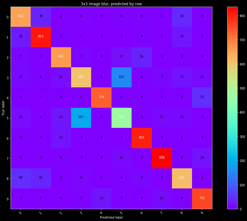
Now, let's fit a model to the rows and columns. We will start by fitting individual models to each set. We use the same grid search for cross validation, on the same data splits. The results are shown in a confusion matrix in Figure 3.
 |
 |
It's clear the predictive power of each of these is limited by themselves. Combining the data yields better results. We fit a model to both the row and column data, and show the results in Figure 4.
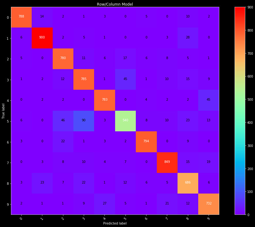
Figure 4: Confusion matrix for predictions on the test data set, from a
Neural Network trained on the normalized sum of rows and columns.
This final row/column combination performs better than each individually. We see a total accuracy of 90%. Not as strong as the image PCA, but still a good performance given the simplicity of the model.
Combined Model
Both of these models show good performance. We thus run a further PCA on the row and column data, selecting only 13 components (96% of the explained variance). This gives us a total of 38 features. We train on the same data as before, but instead use a randomized parameters cross validation. Broadly speaking, randomized cross validation is superior to grid searching, as it does a better job probing parameter space to find optimal hyperparameters. The result is our Scikit-learn model, a neural network with 6 layers.

Figure 5: The final Scikit-Learn model confusion matrix. The model broadly performs
better than the pure img PCA model, but notably predicts more fours as nines.
We end up with a model that has 97% accuracy, the best yet. The only noteable issue is that it seems to predict many fours to be nines, more than in the image PCA only case. If we were building a more complex model we may strive to correct this, but we are doing this primarily as comparison between Sklearn and Tensorflow, so will leave this issue for now.
We continue with model building in the next section, building a model with tensorflow.