Model training
For each team in each game, we have roughly 50 features. We operate under the assumption that each team/game is independent of each other from training purposes, an incorrect assumption but a necessary one.
We take further steps in preparing our training data for machine learning. We z-scale the features to center it on 0 and ensure the standard deviation is 1 for all features, which is necessary for many ML algorithms. Additionally, we implement dimensionality reduction with principal component analysis. The explained variance from the PCA grows slowly, so the reduction is small, but we reduce the number of features to 40 with 90% explained variance.
We test a variety of models, starting with linear models. We first test linear regression and logistic regression, then k nearest neighbors, support vector machines, random forests, and multi layered perceptrons. For each we train on the data from 1999-2019, using a 3 fold cross-validation method to tune hyperparameters. The test data is made up of the 2020-2022 season data, and used for all our metrics unless otherwise stated. For each ML algorithm, we test using either the raw data, scaled input, or PCA reduced data, depending on what makes sense for the model. In most cases, the scaled input was used.
There are a few fields for which we use regression models. The number of rushing yards, passing/receiving yards, and number of complete passes were all fit with regression models. These have a wide range of values, so we will attempt to forecast these values directly.
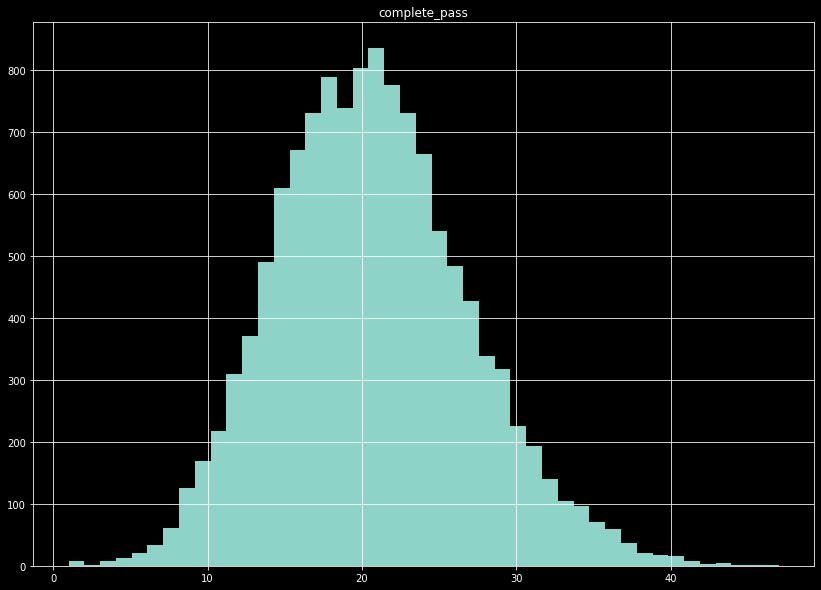
The number of complete passes per game displays a shape similar to the normal distribution.
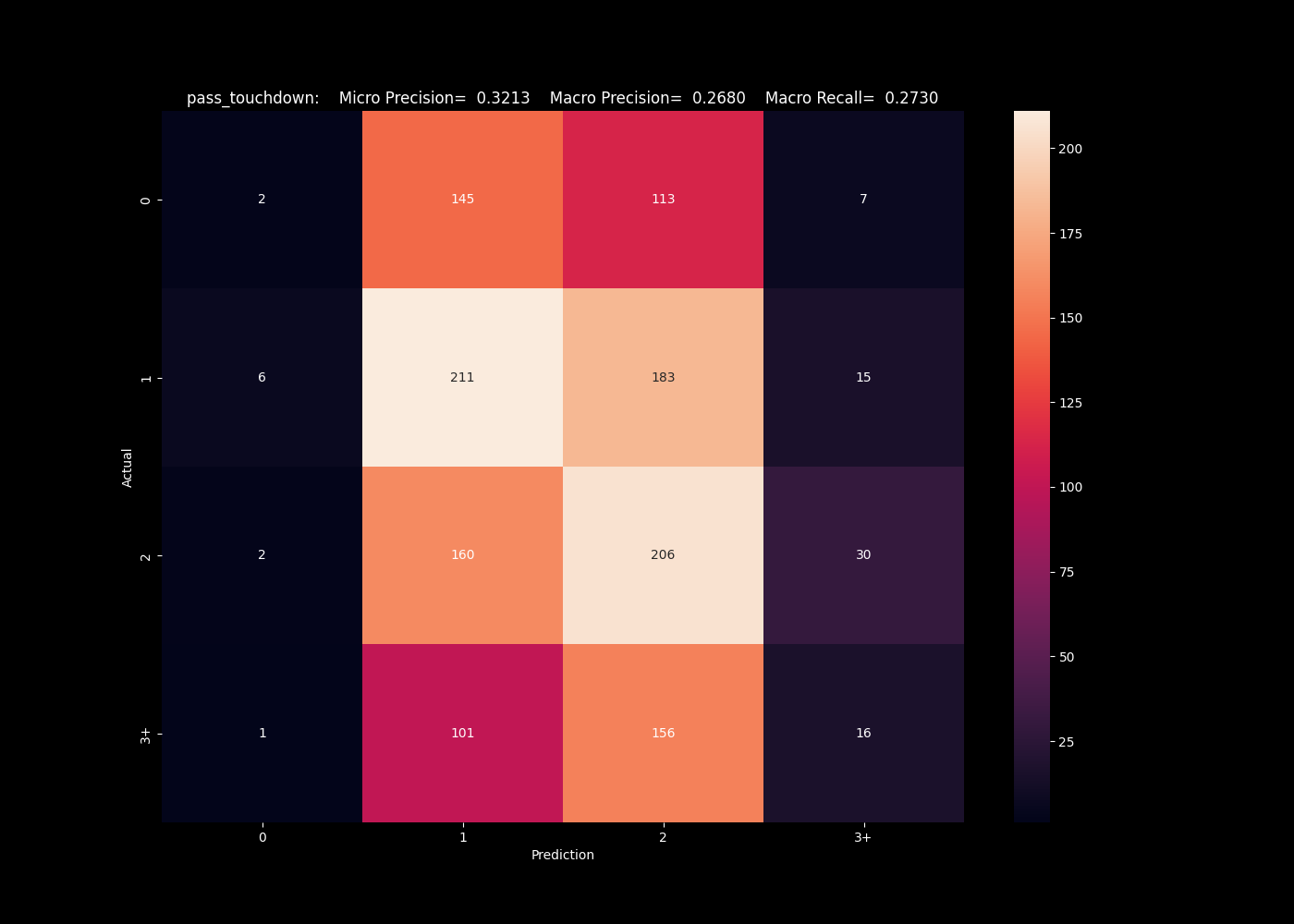
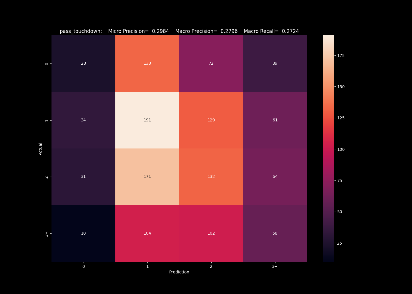
The remaining fields are all binned, and predicted using classification models. For the number of passing touchdowns, for example, drops quickly after 2 passing touchdowns. Since the number of passing touchdowns is a very important metric in fantasy football, we want to be precise, but it is a bit futile to try to predict the high end tail. There are not enough test cases to train the model on this end, so we bin the data to the values 0, 1, 2, and 3+. For the number of touchdowns that exceed 40 yards, the data is so heavily skewed we simply bin as 0 or 1+. In the case of a highly imbalanced data set, we also resample the data such that the majority prediction class is not more than 1.2x the size of the next largest class.
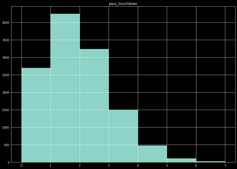
The number of pass touchdowns per game show a tail after ~3 touchdowns.
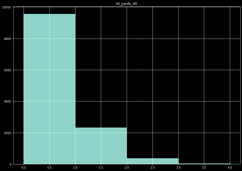
The number of touchdowns over 40 yards per game becomes a binary, 0 or 1+.
Model selection
After training our regressors and classifiers, we compare the results between models to select which we use for our final results.
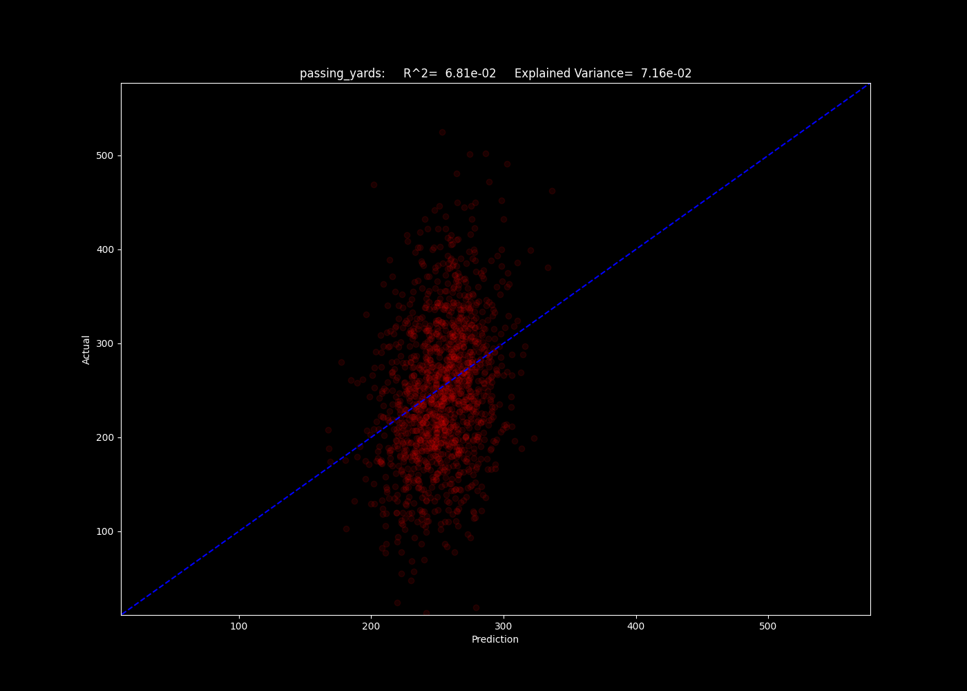
For the regressions, we use the R^2 method to determine which models best fit the predicted yardage and number of pass plays. Below, we show a selection for three of our models of the number of predicted passing yards for games in the 2020-2022 seasons.

The number of passing yards predicted by the linear model. The blue line is a simple 1:1.
The number of passing yards predicted by the multi layered perceptron model.

The number of passing yards predicted by the k neighbors model.
Oof. As we can see, the R^2 values all lie around 0.07, indicating our models explain a small fraction of the trend. The neighbors model may give us insight as to why - the algorithm simply compares an input to the training data closest to it in parameter space. If it performs poorly, this can indicate there is still a significant element of randomness and unpredictability in the results, given the input data. This indicates the input data may not be good at predicting these fields at all.
Moving on to look at classifier categories, we see a much higher rate of success. First, looking at offensive interceptions (interceptions where the team in question threw the ball), we see that the k neighbors algorithm actually does a fair job predicting our categories, of 0/1/2+. We will focus on the macro metrics, which averages the precision across all bins, and see a macro precision of 0.42, meaning our predicted value is correct roughly 42% of the time. This is fairly impressive given the imbalanced in the classes. This imbalance hurts algorithms here such as our neural network, and support vector algorithm, which completely failed to capture the less frequent bins.
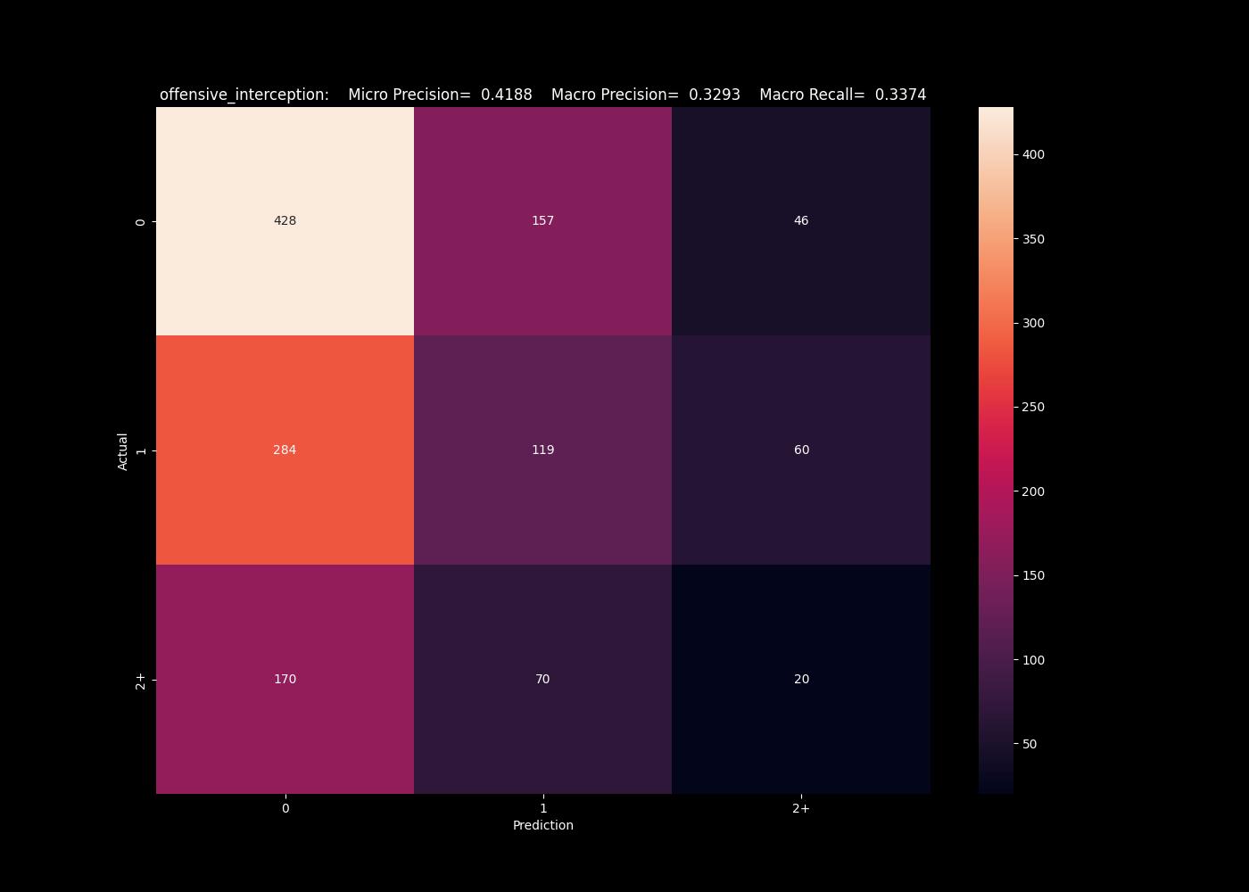
The k nearest neighbors algorithm captures some higher interceptions.
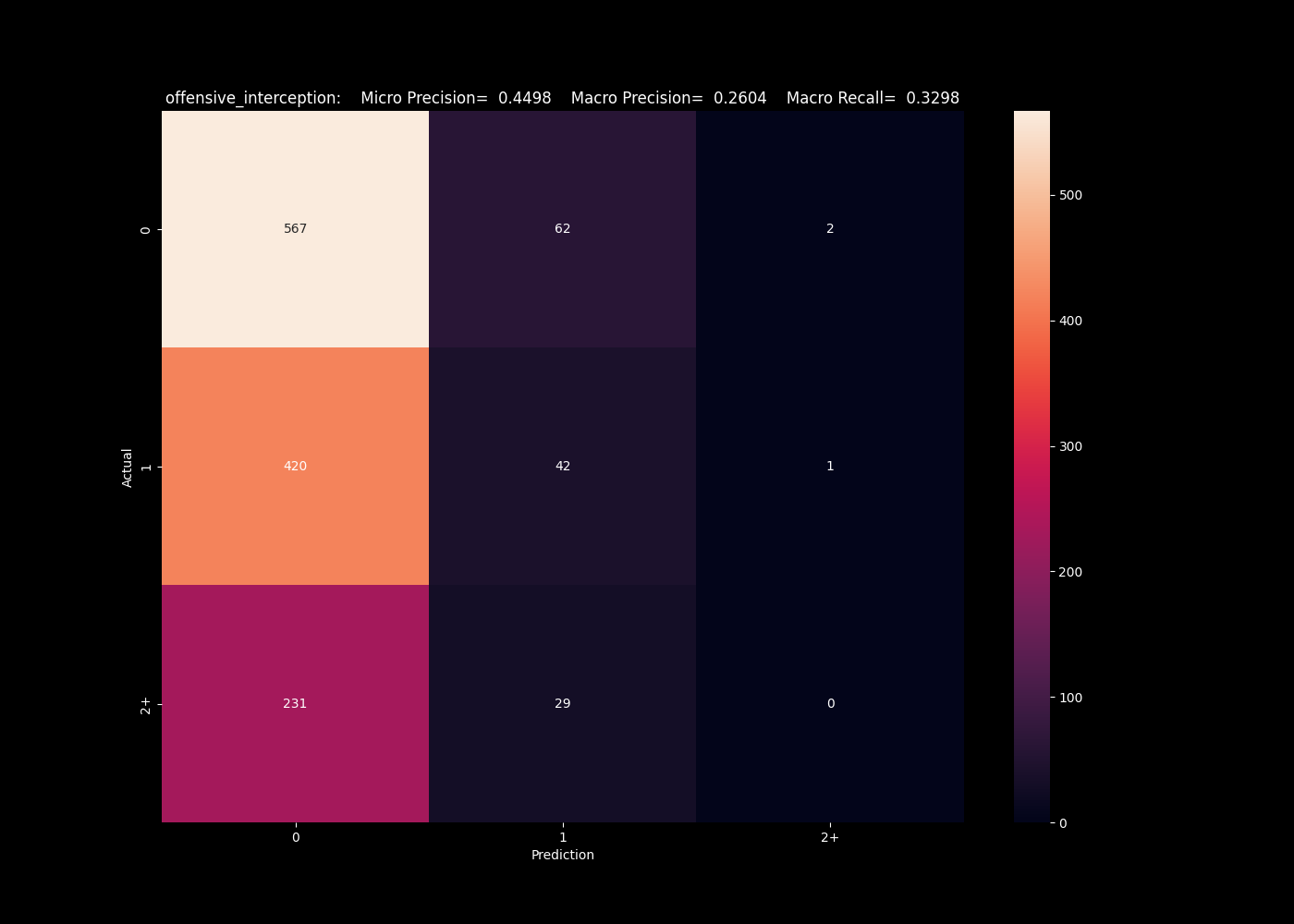
The neural network has a tendency to under predict the numbers of interceptions.
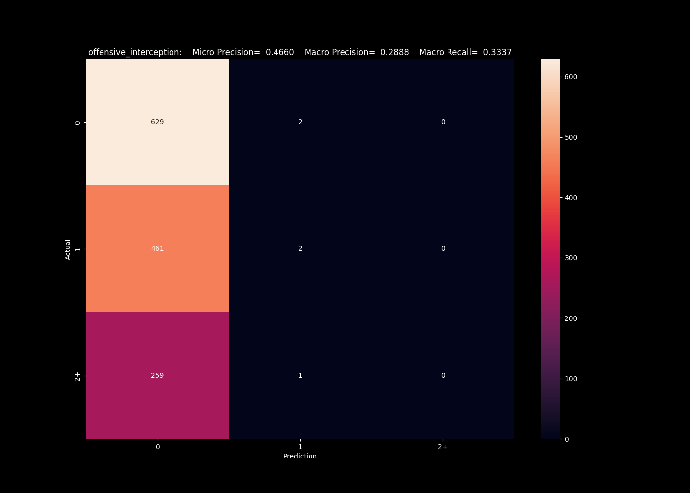
The support vector algorithm completely fails to predict interceptions.
This isn't the only metric with mixed results. For the same algorithms predicting the number of pass touchdowns, we see similar issues predicting values on the edges. Each struggles to predict the edge cases of 0 and 3+, and are imbalanced to the more populated bins.
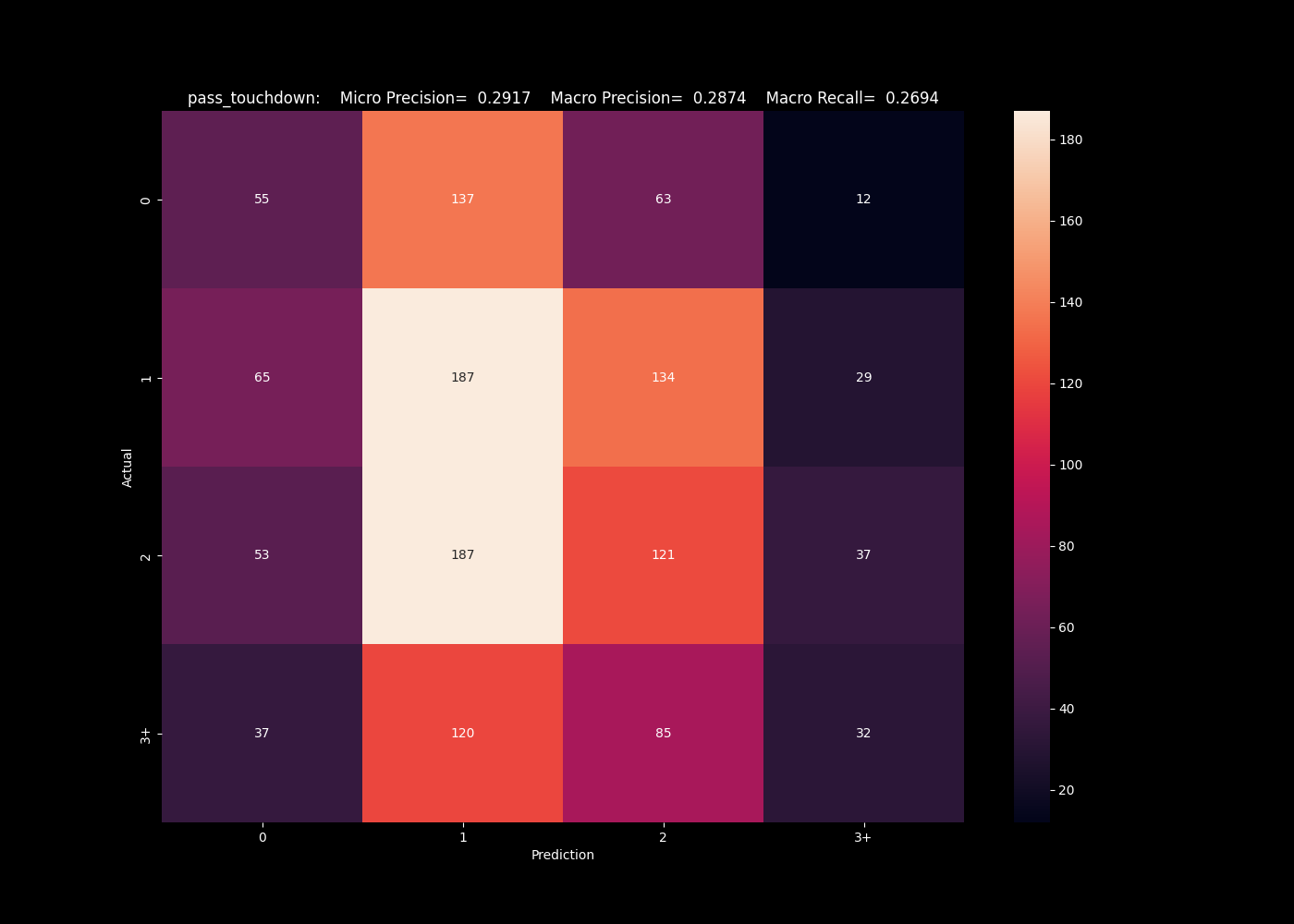
The k nearest neighbors algorithm performs best at predicting the 0 case, but severely under predicts these cases.
 The neural network fails completely to predict the edge bins, favoring the most populous classes.
The support vector algorithm was the worse performer for the offensive interceptions, but here is best at predicting the top end class.
Clearly the strengths and weaknesses of these algorithms are affecting these results. We manually go through each predicted variable to see which algorithm has the best performance, and determine the best regressor model is consistently the linear regression, and use that for our final analysis. The best classifier overall is actually the support vector machine, even though it was a poor performer in our samples above.
Systematic issues in the models
Clearly there are issues with the models ability to forecast. There are a few possible explanations of this. One is a level of randomness from game to game - certainly an effect, but the difference in the model results indicate we should be able to compensate for this on some level.
We already alluded to one issue - data imbalance. Our model all skewed towards the majority class, which is clearly a systemic issue. We could correct this by down sampling further, our current method was just to down sample the largest class to match the second largest. A better scaling would be to scale things to the minority class size, and this will be implemented in later versions. If we implemented this now, we would run into an issue of dimentsionality - with 40-50 fields, we are training models with an extreme number of features. The training data looks at a few tens of thousands of games, and any re-sampling reduces this number. The number of fields we are using is already far too few given the number of records we are using to train. Better re-sampling will come when we implement a more selective sampling on the number of input fields, more specific to each predicted field.
Another factor affecting the results is that of variations in the game over time. We saw in exploration the data is not stationary over time. These trends will affect training and predictions, especially given we are testing on the most recent data. When we downscale the number of fields we train on per predicted value, we will also have an opportunity to train on more recent data to account for this issue.